Simulate System State Trajectories and Measurements
Simulating system state trajectories and measurements requires generative system and measurement equations, e.g., the likelihood function itself is not sufficient. Hence, only the following models can be used for simulation:
For a given system state, the next system state can be simulated by calling the system model's simulate() method. The method draws a random sample from the specified system noise distribution and propagates it together with the given system state through the system equation to obtain a new system state. In a similar manner, a noisy measurement can be generated by calling the measurement model's simulate() method.
Use the model's simulate() class method to simulate system state trajectories or noisy measurements.
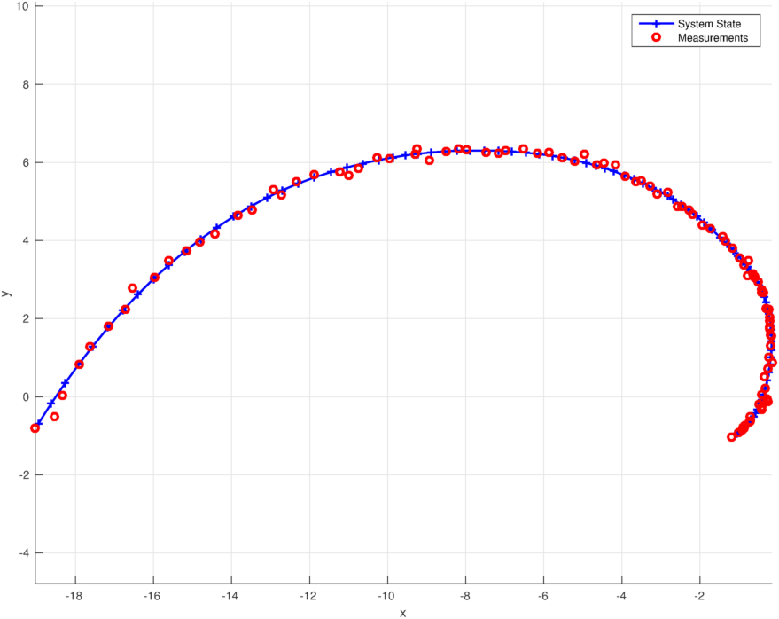
In the following, a target trajectory is simulated over 100 time steps based on the previously introduced TargetSysModel. Additionally, noisy measurements are generated based on the PolarMeasModel.
SimulateTargetAndMeasurements.m
function SimulateTargetAndMeasurements()
    % Instantiate system model
    sysModel = TargetSysModel();

    % Instantiate measurement Model
    measModel = PolarMeasModel();

    % Draw initial system state from the prior state distribution
    initialState = Gaussian([1 1 0 0 0]', [10, 10, 1e-1, 1, 1e-1]);

    sysState = initialState.drawRndSamples(1);

    % Simulate system state trajectory and noisy measurements
    numTimeSteps = 100;

    sysStates    = nan(5, numTimeSteps);
    measurements = nan(2, numTimeSteps);

    for k = 1:numTimeSteps
        % Simulate measurement for time step k
        measurement = measModel.simulate(sysState);

        sysStates(:, k)    = sysState;
        measurements(:, k) = measurement;

        % Simulate next system state
        sysState = sysModel.simulate(sysState);
    end

    figure();
    hold on;
    axis equal;
    grid on;
    xlabel('x');
    ylabel('y');

    % Plot system state trajectory
    plot(sysStates(1, :), sysStates(2, :), 'b-+', 'LineWidth', 1.5, 'DisplayName', 'System State');

    % Plot measurements
    cartMeas = polarToCart(measurements);

    plot(cartMeas(1, :), cartMeas(2, :), 'ro', 'LineWidth', 2, 'DisplayName', 'Measurements');

    legend show;
end

function cartMeas = polarToCart(polarMeas)
    cartMeas = [polarMeas(1, :) .* cos(polarMeas(2, :))
                polarMeas(1, :) .* sin(polarMeas(2, :))];
end
Start the simulation with
>> SimulateTargetAndMeasurements()and you should get a figure like this:
Next, the FilterSet class will be introduced to run and compare several filters for a given estimation problem.