Simulate a Complete State Estimation Problem
Now, we put all things together we learned so far to build a complete simulation of a target tracking problem using the Nonlinear Estimation Toolbox.
The following CompleteEstimationExample() function simulates a random trajectory of target inclusive noisy measurements based on the previously developed system and measurement models. The target will be tracking using different estimators. Relevant data like the true system state, point estimates, or runtimes are collected and subsequently plotted.
You can set for each filter a color/plotting description, e.g., line style, markers, etc., using the setColor() method. It accepts any data like chars or cell arrays. This allows for easy plotting of estimation results. Of course, this functionality can be abused to associate any other data to a filter instance.
CompleteEstimationExample.m
function CompleteEstimationExample()
% Instantiate system model
sysModel = TargetSysModel();
% Instantiate measurement Model
measModel = PolarMeasModel();
% Setup the filters
filters = FilterSet();
filter = EKF();
filter.setColor({ 'Color', [0 0.5 0] });
filters.add(filter);
filter = UKF();
filter.setColor({ 'Color', 'r' });
filters.add(filter);
filter = UKF('Iterative UKF');
filter.setMaxNumIterations(5);
filter.setColor({ 'Color', 'b' });
filters.add(filter);
filter = SIRPF();
filter.setNumParticles(10^5);
filter.setColor({ 'Color', 'm' });
filters.add(filter);
numFilters = filters.getNumFilters();
% Initial state estimate
initialState = Gaussian([1 1 0 0 0]', [10, 10, 1e-1, 1, 1e-1]);
filters.setStates(initialState);
% Simulate system state trajectory and noisy measurements
numTimeSteps = 100;
sysStates = nan(5, numTimeSteps);
measurements = nan(2, numTimeSteps);
updatedStateMeans = nan(5, numFilters, numTimeSteps);
updatedStateCovs = nan(5, 5, numFilters, numTimeSteps);
predStateMeans = nan(5, numFilters, numTimeSteps);
predStateCovs = nan(5, 5, numFilters, numTimeSteps);
runtimesUpdate = nan(numFilters, numTimeSteps);
runtimesPrediction = nan(numFilters, numTimeSteps);
sysState = initialState.drawRndSamples(1);
for k = 1:numTimeSteps
% Simulate measurement for time step k
measurement = measModel.simulate(sysState);
% Save data
sysStates(:, k) = sysState;
measurements(:, k) = measurement;
% Perform measurement update
runtimesUpdate(:, k) = filters.update(measModel, measurement);
[updatedStateMeans(:, :, k), ...
updatedStateCovs(:, :, :, k)] = filters.getStatesMeanAndCov();
% Simulate next system state
sysState = sysModel.simulate(sysState);
% Perform state prediction
runtimesPrediction(:, k) = filters.predict(sysModel);
[predStateMeans(:, :, k), ...
predStateCovs(:, :, :, k)] = filters.getStatesMeanAndCov();
end
close all;
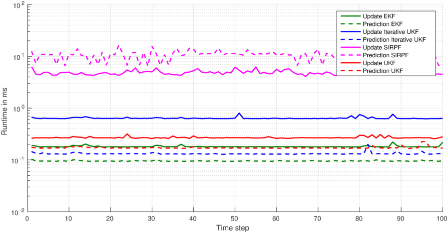
% Plot state prediction and measurement update runtimes
figure();
hold on;
grid on;
xlabel('Time step');
ylabel('Runtime in ms');
for i = 1:numFilters
filter = filters.get(i);
color = filter.getColor();
name = filter.getName();
r = runtimesUpdate(i, :) * 1000;
plot(1:numTimeSteps, r, '-', 'LineWidth', 1.5, color{:}, ...
'DisplayName', sprintf('Update %s', name));
r = runtimesPrediction(i, :) * 1000;
plot(1:numTimeSteps, r, '--', 'LineWidth', 1.5, color{:}, ...
'DisplayName', sprintf('Prediction %s', name));
end
set(gca, 'yscale', 'log');
legend show;
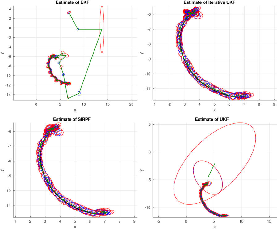
% Plot state estimates
figure();
for i = 1:numFilters
subplot(2, 2, i);
hold on;
axis equal;
grid on;
xlabel('x');
ylabel('y');
filter = filters.get(i);
name = filter.getName();
title(['Estimate of ' name]);
% Plot true system state
plot(sysStates(1, :), sysStates(2, :), 'k-', 'LineWidth', 2);
% Show confidence interval of 99%
confidence = 0.99;
objectTrace = nan(2, 2 * numTimeSteps);
j = 1;
for k = 1:numTimeSteps
% Plot updated estimate
updatedPosMean = updatedStateMeans(1:2, i, k);
updatedPosCov = updatedStateCovs(1:2, 1:2, i, k);
plotCovariance(updatedPosMean, updatedPosCov, confidence, 'b-');
objectTrace(:, j) = updatedPosMean;
j = j + 1;
% Plot predicted estimate
predPosMean = predStateMeans(1:2, i, k);
predPosCov = predStateCovs(1:2, 1:2, i, k);
plotCovariance(predPosMean, predPosCov, confidence, 'r-');
objectTrace(:, j) = predPosMean;
j = j + 1;
end
% Plot object trace
plot(objectTrace(1, :), objectTrace(2, :), 'Color', [0 0.5 0], 'LineWidth', 1);
end
end
function handle = plotCovariance(mean, covariance, confidence, varargin)
% covariance = V * D * V'
[V, D] = eig(covariance);
sigma = sqrt(diag(D));
scaling = sqrt(chi2inv(confidence, 2));
if covariance(1, 1) > covariance(2, 2)
phi = atan2(V(2, 2), V(1, 2));
extent = scaling * [sigma(2) sigma(1)];
else
phi = atan2(V(2, 1), V(1, 1));
extent = scaling * [sigma(1) sigma(2)];
end
handle = plotEllipse(mean, extent, phi, varargin{:});
end
function handle = plotEllipse(center, extent, angle, varargin)
a = 0:0.01:2*pi;
s = [extent(1) * cos(a)
extent(2) * sin(a)];
ca = cos(angle);
sa = sin(angle);
s = [ca -sa
sa ca] * s;
handle = plot([s(1, :) s(1, 1)] + center(1), [s(2, :) s(2, 1)] + center(2), varargin{:});
endExecuting the file with
>> CompleteEstimationExample()and you should get figures like this:
At this point, you are familiar with the basic principles of the Nonlinear Estimation Toolbox! Now, you should have a look at the complete list of Estimators available in the toolbox or get an overview of the Probability Distributions, System Models, and Measurement Models not treated here.