Gaussian Sampling Example

function GaussianSamplingExample()
    % An illustrative example how to use the GaussianSampling (sub)classes
    
    % This example demonstrates the usage of the implemented Gaussian
    % sampling techniques. As all samplings possess a common interface
    % for drawing samples of standard normal and arbitrary Gaussian
    % distributions, they can be easily exchanged or their performance
    % compared.
    
    % Each sampling has its own methods (if any provided) for setting up
    % the respective sampling techniques. For example, the sample spread of
    % the UKF, or the number of samples for the Gaussian LCD sampling and
    % the simple random sampling.
    
    % Moreover, if a new Gaussian sampling technique will be implemented
    % in the same manner, it can be easily exchanged with existing sampling
    % techniques without any significant changes to the existing code.
    
    
    % Setup Gaussian sampling techniques ...
    
    % Sampling from the Unscented KF with
    % double weighted sample at the origin
    samplings{1}.name = 'UKF';
    samplings{1}.sampling = GaussianSamplingUKF();
    samplings{1}.sampling.setSampleScaling(1);
    
    % Sampling from the 5th-Degree Cubature KF
    samplings{2}.name = '5th-Degree CKF';
    samplings{2}.sampling = GaussianSamplingCKF();
    
    % Symmetric Gaussian LCD sampling (from the S2KF / PGF) with 21 samples
    samplings{3}.name = 'Symmetric LCD';
    samplings{3}.sampling = GaussianSamplingLCD();
    samplings{3}.sampling.setNumSamplesByFactor(10);
    
    % Aymmetric Gaussian LCD sampling (from the S2KF / PGF) with 21 samples
    samplings{4}.name = 'Asymmetric LCD';
    samplings{4}.sampling = GaussianSamplingLCD();
    samplings{4}.sampling.setSymmetricMode(false);
    samplings{4}.sampling.setNumSamples(21);
    
    % Sampling from the Randomized UKF using 10 iterations
    samplings{5}.name = 'RUKF';
    samplings{5}.sampling = GaussianSamplingRUKF();
    samplings{5}.sampling.setNumIterations(10);
    
    % Sampling from the Gauss-Hermite Kalman Filter
    % with 3 quadrature points per dimension
    samplings{6}.name = 'Gauss-Hermite';
    samplings{6}.sampling = GaussianSamplingGHQ();
    samplings{6}.sampling.setNumQuadraturePoints(3);
    
    % Finally, simple random sampling with 100 samples
    samplings{7}.name = 'Random';
    samplings{7}.sampling = GaussianSamplingRnd();
    samplings{7}.sampling.setNumSamples(100);
    
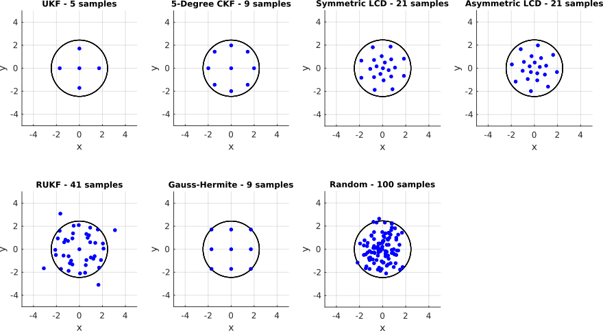
    % ... and plot their respecitve samples in the 2D case ...
    
    % ... for the standard normal distribution ...
    plotSamplings(samplings);
    
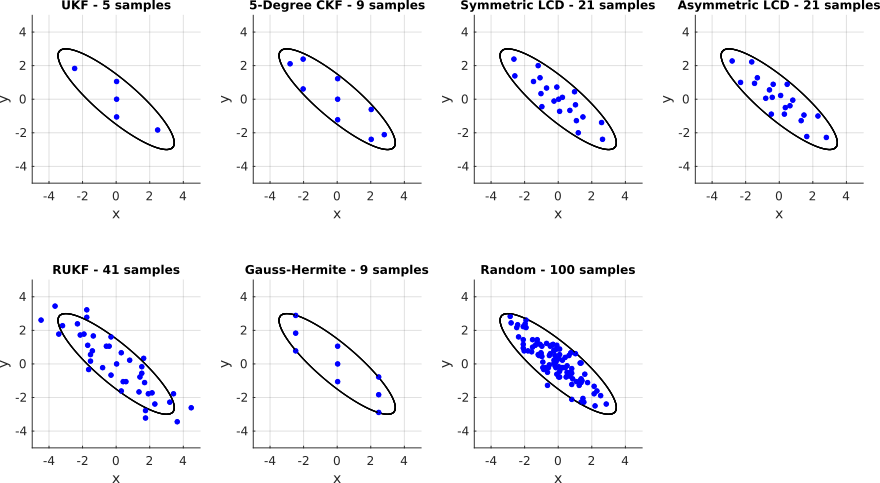
    % ... and for a 2D non-standard Gaussian.
    mean       = [0 0]';
    covariance = [ 2.0 -1.5
                  -1.5  1.5];
    gaussian   = Gaussian(mean, covariance);
    
    % By changing the view of each plot one can see the different
    % sample weightings for different sampling techniques.
    
    plotSamplings(samplings, gaussian);
end

function plotSamplings(samplings, gaussian)
    figure();
    
    % Iterate through all sampling techniques
    for i = 1:numel(samplings)
        subplot(2, 4, i);
        
        % Setup sub plot
        hold on;
        xlabel('x');
        ylabel('y');
        zlabel('Weight');
        grid on;
        axis equal;
        set(gca, 'XTick', -4:2:4);
        set(gca, 'YTick', -4:2:4);
        set(gca, 'XLim', [-5, 5]);
        set(gca, 'YLim', [-5, 5]);
        set(gca, 'ZLim', [-5, 5]);
        
        % Select between standard normal and non-standard case
        if nargin == 1
            % Sample from the 2D standard normal distribution
            [samples, weights, numSamples] = samplings{i}.sampling.getStdNormalSamples(2);
            
            % For drawing confidence interval
            mean = zeros(2, 1);
            covariance = eye(2);
        else
            % Sample from the given Gaussian distribution
            [samples, weights, numSamples] = samplings{i}.sampling.getSamples(gaussian);
            
            % For drawing confidence interval
            [mean, covariance] = gaussian.getMeanAndCov();
        end
        
        % Set sampling plot title
        title(sprintf('%s - %d samples', samplings{i}.name, numSamples), 'FontSize', 10);
        
        % For better visualization, all weights get scaled
        % so that the maximum weight is at a value of 6.
        % By changing the view of each plot one can see the different
        % sample weightings for different sampling techniques.
        weights = 5 * weights / max(abs(weights));
        
        if numel(weights) == 1
            % Gaussian sampling techniques only return a single scalar
            % weight in case of equally weighted samples. Hence, for the
            % visualization we have to repmat the weight
            weights = repmat(weights, 1, numSamples);
        end
        
        % Plot weighted samples from sampling #i
        stem3(samples(1, :), samples(2, :), weights, ...
             'bo', 'LineWidth', 2, 'MarkerSize', 2);
        
        % Draw confidence interval of 95%
        plotCovariance(mean, covariance, 0.95, 'k-', 'LineWidth', 1);
    end
end

function handle = plotCovariance(mean, covariance, confidence, varargin)
    % covariance = V * D * V'
    [V, D] = eig(covariance);
    
    sigma = sqrt(diag(D));
    
    phi = atan2(V(2, 1), V(1, 1));
    
    scaling = sqrt(chi2inv(confidence, 2));
    
    extent = scaling * [sigma(1) sigma(2)];
    
    handle = plotEllipse(mean, extent, phi, varargin{:});
end

function handle = plotEllipse(center, extent, angle, varargin)
    a = 0:0.01:2*pi;
    
    s = [extent(1) * cos(a)
         extent(2) * sin(a)];
    
    ca = cos(angle);
    sa = sin(angle);
    
    s = [ca -sa
         sa  ca] * s;
    
    handle = plot(s(1, :) + center(1), s(2, :) + center(2), varargin{:});
end